Python Tutorial
II. Linear Systems of Ordinary Differential Equations
1. Systems of ordinary differential equations
Systems of ODEs appear naturally when modeling interconnected phenomena. Let's explore how to solve and visualize them:
import numpy as np
import matplotlib.pyplot as plt
from scipy.integrate import odeint, solve_ivp
from matplotlib.animation import FuncAnimation

# Example 1: Coupled oscillators (mass-spring system)
print("Coupled Mass-Spring System")
print("=========================")

# System: Two masses connected by springs
# m1*x1'' = -k1*x1 + k2*(x2 - x1)
# m2*x2'' = -k2*(x2 - x1)

# Convert to first order: [x1, v1, x2, v2]
def coupled_oscillators(t, y):
    x1, v1, x2, v2 = y
    m1, m2 = 1.0, 1.0  # masses
    k1, k2 = 3.0, 2.0  # spring constants

    dx1dt = v1
    dv1dt = (-k1*x1 + k2*(x2 - x1)) / m1
    dx2dt = v2
    dv2dt = -k2*(x2 - x1) / m2

    return [dx1dt, dv1dt, dx2dt, dv2dt]

# Initial conditions: x1=1, v1=0, x2=0, v2=0
y0 = [1.0, 0.0, 0.0, 0.0]
t_span = (0, 20)
t_eval = np.linspace(0, 20, 1000)

# Solve the system
sol = solve_ivp(coupled_oscillators, t_span, y0, t_eval=t_eval)

# Plot results
fig, axes = plt.subplots(2, 2, figsize=(12, 10))

# Position vs time
ax1 = axes[0, 0]
ax1.plot(sol.t, sol.y[0], 'b-', label='Mass 1')
ax1.plot(sol.t, sol.y[2], 'r-', label='Mass 2')
ax1.set_xlabel('Time')
ax1.set_ylabel('Position')
ax1.set_title('Positions vs Time')
ax1.legend()
ax1.grid(True, alpha=0.3)

# Phase portrait for mass 1
ax2 = axes[0, 1]
ax2.plot(sol.y[0], sol.y[1], 'b-', alpha=0.7)
ax2.scatter(y0[0], y0[1], color='green', s=100, marker='o', label='Start')
ax2.set_xlabel('Position (x1)')
ax2.set_ylabel('Velocity (v1)')
ax2.set_title('Phase Portrait - Mass 1')
ax2.legend()
ax2.grid(True, alpha=0.3)

# Configuration space
ax3 = axes[1, 0]
ax3.plot(sol.y[0], sol.y[2], 'purple', alpha=0.7)
ax3.scatter(y0[0], y0[2], color='green', s=100, marker='o', label='Start')
ax3.set_xlabel('Position x1')
ax3.set_ylabel('Position x2')
ax3.set_title('Configuration Space (x1 vs x2)')
ax3.legend()
ax3.grid(True, alpha=0.3)
ax3.set_aspect('equal')

# Energy analysis
ax4 = axes[1, 1]
m1, m2, k1, k2 = 1.0, 1.0, 3.0, 2.0
KE = 0.5*m1*sol.y[1]**2 + 0.5*m2*sol.y[3]**2  # Kinetic energy
PE = 0.5*k1*sol.y[0]**2 + 0.5*k2*(sol.y[2]-sol.y[0])**2  # Potential energy
TE = KE + PE  # Total energy

ax4.plot(sol.t, KE, 'b-', label='Kinetic Energy')
ax4.plot(sol.t, PE, 'r-', label='Potential Energy')
ax4.plot(sol.t, TE, 'k--', label='Total Energy', linewidth=2)
ax4.set_xlabel('Time')
ax4.set_ylabel('Energy')
ax4.set_title('Energy Conservation')
ax4.legend()
ax4.grid(True, alpha=0.3)

plt.tight_layout()
plt.show()

# Example 2: Predator-Prey System (Lotka-Volterra)
print("\nLotka-Volterra Predator-Prey Model")
print("===================================")

def lotka_volterra(t, y):
    prey, predator = y
    alpha = 1.0    # prey growth rate
    beta = 0.1     # predation rate
    gamma = 1.5    # predator death rate
    delta = 0.075  # predator efficiency

    dprey_dt = alpha*prey - beta*prey*predator
    dpredator_dt = delta*prey*predator - gamma*predator

    return [dprey_dt, dpredator_dt]

# Different initial conditions
initial_conditions = [
    [10, 5],   # Normal
    [15, 5],   # More prey
    [10, 10],  # More predators
    [25, 15]   # Both high
]

fig, (ax1, ax2) = plt.subplots(1, 2, figsize=(14, 6))

colors = ['blue', 'green', 'red', 'purple']
t_span = (0, 50)
t_eval = np.linspace(0, 50, 1000)

for ic, color in zip(initial_conditions, colors):
    sol = solve_ivp(lotka_volterra, t_span, ic, t_eval=t_eval)

    # Time series
    ax1.plot(sol.t, sol.y[0], color=color, linestyle='-',
             label=f'Prey (IC: {ic})', alpha=0.7)
    ax1.plot(sol.t, sol.y[1], color=color, linestyle='--',
             label=f'Predator (IC: {ic})', alpha=0.7)

    # Phase portrait
    ax2.plot(sol.y[0], sol.y[1], color=color, alpha=0.7)
    ax2.scatter(ic[0], ic[1], color=color, s=100, marker='o')

ax1.set_xlabel('Time')
ax1.set_ylabel('Population')
ax1.set_title('Population Dynamics')
ax1.legend(bbox_to_anchor=(1.05, 1), loc='upper left')
ax1.grid(True, alpha=0.3)

ax2.set_xlabel('Prey Population')
ax2.set_ylabel('Predator Population')
ax2.set_title('Phase Portrait')
ax2.grid(True, alpha=0.3)

plt.tight_layout()
plt.show()

# Example 3: Linear system in matrix form
print("\nLinear System: dx/dt = Ax")
print("==========================")

# Define matrix A
A = np.array([[-0.5, 2.0],
              [-2.0, -0.5]])

print("System matrix A:")
print(A)

# Eigenvalue analysis
eigenvalues, eigenvectors = np.linalg.eig(A)
print(f"\nEigenvalues: {eigenvalues}")
print(f"Eigenvectors:\n{eigenvectors}")

# Classify the system
if np.all(np.real(eigenvalues) < 0):
    if np.all(np.imag(eigenvalues) == 0):
        stability = "Stable node"
    else:
        stability = "Stable spiral"
elif np.all(np.real(eigenvalues) > 0):
    if np.all(np.imag(eigenvalues) == 0):
        stability = "Unstable node"
    else:
        stability = "Unstable spiral"
elif np.real(eigenvalues[0]) * np.real(eigenvalues[1]) < 0:
    stability = "Saddle point"
else:
    stability = "Center"

print(f"\nSystem type: {stability}")

# Solve and visualize
def linear_system(t, y):
    return A @ y

# Multiple trajectories
fig, ax = plt.subplots(figsize=(8, 8))

# Create initial conditions on a circle
n_trajectories = 20
theta = np.linspace(0, 2*np.pi, n_trajectories)

for i in range(n_trajectories):
    r = 2.0
    ic = [r*np.cos(theta[i]), r*np.sin(theta[i])]

    sol = solve_ivp(linear_system, (0, 10), ic, t_eval=np.linspace(0, 10, 500))

    ax.plot(sol.y[0], sol.y[1], 'b-', alpha=0.5, linewidth=1)
    ax.scatter(ic[0], ic[1], color='red', s=30)

# Plot eigenvector directions
for i in range(2):
    v = eigenvectors[:, i]
    if np.isreal(eigenvalues[i]):
        scale = 3
        ax.arrow(0, 0, scale*v[0], scale*v[1], head_width=0.2,
                 head_length=0.1, fc='green', ec='green', linewidth=2)
        ax.text(scale*v[0]*1.2, scale*v[1]*1.2,
                f'λ={eigenvalues[i]:.2f}', fontsize=12)

ax.set_xlim(-3, 3)
ax.set_ylim(-3, 3)
ax.set_aspect('equal')
ax.grid(True, alpha=0.3)
ax.set_xlabel('x')
ax.set_ylabel('y')
ax.set_title(f'Phase Portrait: {stability}')

plt.show()
2. Constant coefficient equations
For systems with constant coefficients, we can find analytical solutions using eigenvalues and eigenvectors:
import numpy as np
import matplotlib.pyplot as plt
from scipy.linalg import expm
import sympy as sp

# Example: Solve dx/dt = Ax with x(0) = x0
print("Solving Constant Coefficient Systems")
print("===================================\n")

# Define the system matrix
A = np.array([[1, 2],
              [3, 2]])

x0 = np.array([1, 0])  # Initial condition

print("System: dx/dt = Ax")
print("A =")
print(A)
print("\nInitial condition x0 =", x0)

# Method 1: Using eigenvalues and eigenvectors
eigenvalues, eigenvectors = np.linalg.eig(A)
print("\nEigenvalues:", eigenvalues)
print("Eigenvectors:")
print(eigenvectors)

# General solution: x(t) = c1*v1*exp(λ1*t) + c2*v2*exp(λ2*t)
# Find coefficients c1, c2 from initial condition
coeffs = np.linalg.solve(eigenvectors, x0)
print("\nCoefficients c =", coeffs)

# Create solution function
def analytical_solution(t):
    x = np.zeros((len(t), 2))
    for i in range(len(t)):
        x[i] = (coeffs[0] * eigenvectors[:, 0] * np.exp(eigenvalues[0] * t[i]) +
                coeffs[1] * eigenvectors[:, 1] * np.exp(eigenvalues[1] * t[i])).real
    return x

# Method 2: Using matrix exponential
# Solution: x(t) = exp(At) * x0
def matrix_exp_solution(t):
    x = np.zeros((len(t), 2))
    for i in range(len(t)):
        x[i] = expm(A * t[i]) @ x0
    return x

# Time array
t = np.linspace(0, 2, 100)

# Compute solutions
x_analytical = analytical_solution(t)
x_matrix_exp = matrix_exp_solution(t)

# Verify they match
print("\nMax difference between methods:",
      np.max(np.abs(x_analytical - x_matrix_exp)))

# Visualization
fig, axes = plt.subplots(2, 2, figsize=(12, 10))

# Time series
ax1 = axes[0, 0]
ax1.plot(t, x_analytical[:, 0], 'b-', label='x1(t)', linewidth=2)
ax1.plot(t, x_analytical[:, 1], 'r-', label='x2(t)', linewidth=2)
ax1.set_xlabel('Time t')
ax1.set_ylabel('x(t)')
ax1.set_title('Solution Components vs Time')
ax1.legend()
ax1.grid(True, alpha=0.3)

# Phase portrait
ax2 = axes[0, 1]
ax2.plot(x_analytical[:, 0], x_analytical[:, 1], 'purple', linewidth=2)
ax2.scatter(x0[0], x0[1], color='green', s=100, marker='o',
            label='Initial condition', zorder=5)
ax2.set_xlabel('x1')
ax2.set_ylabel('x2')
ax2.set_title('Phase Portrait')
ax2.legend()
ax2.grid(True, alpha=0.3)
ax2.set_aspect('equal')

# Direction field
ax3 = axes[1, 0]
x1_range = np.linspace(-2, 3, 20)
x2_range = np.linspace(-2, 3, 20)
X1, X2 = np.meshgrid(x1_range, x2_range)

# Compute direction vectors
DX1 = A[0, 0] * X1 + A[0, 1] * X2
DX2 = A[1, 0] * X1 + A[1, 1] * X2

# Normalize
M = np.sqrt(DX1**2 + DX2**2)
DX1_norm = DX1 / M
DX2_norm = DX2 / M

ax3.quiver(X1, X2, DX1_norm, DX2_norm, M, cmap='viridis', alpha=0.6)
ax3.plot(x_analytical[:, 0], x_analytical[:, 1], 'red', linewidth=2)
ax3.scatter(x0[0], x0[1], color='red', s=100, marker='o', zorder=5)
ax3.set_xlabel('x1')
ax3.set_ylabel('x2')
ax3.set_title('Direction Field with Solution')
ax3.set_xlim(-2, 3)
ax3.set_ylim(-2, 3)

# Matrix exponential visualization
ax4 = axes[1, 1]
t_values = [0, 0.5, 1, 1.5, 2]
colors = plt.cm.viridis(np.linspace(0, 1, len(t_values)))

for i, t_val in enumerate(t_values):
    exp_At = expm(A * t_val)

    # Show how unit circle transforms
    theta = np.linspace(0, 2*np.pi, 100)
    unit_circle = np.array([np.cos(theta), np.sin(theta)])
    transformed = exp_At @ unit_circle

    ax4.plot(transformed[0], transformed[1], color=colors[i],
             label=f't = {t_val}', linewidth=2)

ax4.set_xlabel('x1')
ax4.set_ylabel('x2')
ax4.set_title('Evolution of Unit Circle under exp(At)')
ax4.legend()
ax4.grid(True, alpha=0.3)
ax4.set_aspect('equal')
ax4.set_xlim(-10, 10)
ax4.set_ylim(-10, 10)

plt.tight_layout()
plt.show()

# Complex eigenvalues example
print("\n" + "="*50)
print("System with Complex Eigenvalues")
print("="*50)

# Rotation + scaling matrix
A_complex = np.array([[0.5, -2],
                      [2, 0.5]])

print("\nMatrix A:")
print(A_complex)

eig_vals, eig_vecs = np.linalg.eig(A_complex)
print("\nEigenvalues:", eig_vals)
print("Real parts:", np.real(eig_vals))
print("Imaginary parts:", np.imag(eig_vals))

# Solve with different initial conditions
fig, (ax1, ax2) = plt.subplots(1, 2, figsize=(12, 5))

initial_conditions = [[1, 0], [0, 1], [1, 1], [-1, 1]]
colors = ['blue', 'red', 'green', 'purple']

t = np.linspace(0, 5, 500)

for ic, color in zip(initial_conditions, colors):
    x = np.zeros((len(t), 2))
    for i in range(len(t)):
        x[i] = expm(A_complex * t[i]) @ ic

    ax1.plot(t, x[:, 0], color=color, linestyle='-',
             label=f'x1, IC={ic}', alpha=0.7)
    ax1.plot(t, x[:, 1], color=color, linestyle='--',
             label=f'x2, IC={ic}', alpha=0.7)

    ax2.plot(x[:, 0], x[:, 1], color=color, alpha=0.7)
    ax2.scatter(ic[0], ic[1], color=color, s=100, marker='o')

ax1.set_xlabel('Time')
ax1.set_ylabel('x(t)')
ax1.set_title('Spiral Solutions (Complex Eigenvalues)')
ax1.legend(bbox_to_anchor=(1.05, 1), loc='upper left')
ax1.grid(True, alpha=0.3)

ax2.set_xlabel('x1')
ax2.set_ylabel('x2')
ax2.set_title('Spiral Phase Portrait')
ax2.grid(True, alpha=0.3)
ax2.set_aspect('equal')

plt.tight_layout()
plt.show()

# Symbolic solution using SymPy
print("\n" + "="*50)
print("Symbolic Solution using SymPy")
print("="*50)

t = sp.Symbol('t')
A_sym = sp.Matrix([[1, 2], [3, 2]])
x0_sym = sp.Matrix([1, 0])

print("\nComputing matrix exponential symbolically...")
exp_At = sp.exp(A_sym * t)

print("\nexp(At) =")
sp.pprint(exp_At)

# Solution
x_sym = exp_At * x0_sym
print("\nSolution x(t) = exp(At) * x0:")
sp.pprint(x_sym)
3. Direction Fields
Direction fields (slope fields) provide visual insight into the behavior of differential equation systems:
import numpy as np
import matplotlib.pyplot as plt
from matplotlib.patches import FancyArrowPatch
import matplotlib.colors as mcolors

# Create interactive direction field visualizer
print("Direction Field Visualization for Linear Systems")
print("===============================================\n")

# Different types of linear systems
systems = {
    'Stable Node': np.array([[-2, 0], [0, -1]]),
    'Unstable Node': np.array([[2, 0], [0, 1]]),
    'Saddle Point': np.array([[1, 0], [0, -2]]),
    'Center': np.array([[0, -2], [2, 0]]),
    'Stable Spiral': np.array([[-0.5, -2], [2, -0.5]]),
    'Unstable Spiral': np.array([[0.5, -2], [2, 0.5]])
}

fig, axes = plt.subplots(2, 3, figsize=(15, 10))
axes = axes.ravel()

for idx, (name, A) in enumerate(systems.items()):
    ax = axes[idx]

    # Create grid
    x = np.linspace(-3, 3, 20)
    y = np.linspace(-3, 3, 20)
    X, Y = np.meshgrid(x, y)

    # Compute direction field
    U = A[0, 0] * X + A[0, 1] * Y
    V = A[1, 0] * X + A[1, 1] * Y

    # Compute speed for coloring
    speed = np.sqrt(U**2 + V**2)

    # Normalize arrows
    U_norm = U / (speed + 0.001)
    V_norm = V / (speed + 0.001)

    # Plot direction field
    quiver = ax.quiver(X, Y, U_norm, V_norm, speed,
                       cmap='coolwarm', alpha=0.8, scale=25)

    # Add some solution trajectories
    from scipy.integrate import odeint

    def system(state, t):
        return A @ state

    # Initial conditions
    for angle in np.linspace(0, 2*np.pi, 8, endpoint=False):
        x0 = 2 * np.array([np.cos(angle), np.sin(angle)])
        t = np.linspace(0, 5, 500)

        try:
            trajectory = odeint(system, x0, t)
            # Only plot if trajectory doesn't diverge too much
            if np.max(np.abs(trajectory)) < 10:
                ax.plot(trajectory[:, 0], trajectory[:, 1],
                       'k-', linewidth=1, alpha=0.5)
                ax.plot(x0[0], x0[1], 'go', markersize=4)
        except:
            pass

    # Eigenvalues and eigenvectors
    eigenvalues, eigenvectors = np.linalg.eig(A)

    # Plot eigenvector directions if real
    for i in range(2):
        if np.abs(np.imag(eigenvalues[i])) < 1e-10:
            v = eigenvectors[:, i].real
            # Plot both directions
            for sign in [-1, 1]:
                ax.arrow(0, 0, sign*v[0], sign*v[1],
                        head_width=0.15, head_length=0.1,
                        fc='red', ec='red', linewidth=2, alpha=0.7)

    ax.set_xlim(-3, 3)
    ax.set_ylim(-3, 3)
    ax.set_aspect('equal')
    ax.grid(True, alpha=0.3)
    ax.set_title(f'{name}\nλ = {eigenvalues}', fontsize=12)
    ax.set_xlabel('x')
    ax.set_ylabel('y')

plt.tight_layout()
plt.show()

# Interactive direction field explorer
print("\n" + "="*50)
print("Nonlinear System Direction Fields")
print("="*50)

# Nonlinear examples
def van_der_pol(state, mu=1.0):
    x, y = state
    dxdt = y
    dydt = mu * (1 - x**2) * y - x
    return np.array([dxdt, dydt])

def duffing(state, alpha=1.0, beta=0.1):
    x, y = state
    dxdt = y
    dydt = -alpha * x - beta * x**3
    return np.array([dxdt, dydt])

def predator_prey(state, a=1.0, b=0.1, c=1.5, d=0.075):
    x, y = state
    dxdt = a*x - b*x*y
    dydt = d*x*y - c*y
    return np.array([dxdt, dydt])

# Visualize nonlinear systems
fig, axes = plt.subplots(1, 3, figsize=(15, 5))

systems_nonlinear = [
    ('Van der Pol Oscillator', van_der_pol, (-3, 3), (-3, 3)),
    ('Duffing Oscillator', duffing, (-3, 3), (-3, 3)),
    ('Predator-Prey', predator_prey, (0, 40), (0, 20))
]

for ax, (name, func, xlim, ylim) in zip(axes, systems_nonlinear):
    # Create appropriate grid
    x = np.linspace(xlim[0], xlim[1], 25)
    y = np.linspace(ylim[0], ylim[1], 25)
    X, Y = np.meshgrid(x, y)

    # Compute direction field
    U = np.zeros_like(X)
    V = np.zeros_like(Y)

    for i in range(X.shape[0]):
        for j in range(X.shape[1]):
            state = np.array([X[i, j], Y[i, j]])
            derivative = func(state)
            U[i, j] = derivative[0]
            V[i, j] = derivative[1]

    # Speed for coloring
    speed = np.sqrt(U**2 + V**2)

    # Plot streamlines instead of quiver for smoother visualization
    strm = ax.streamplot(x, y, U.T, V.T, color=speed.T,
                         cmap='viridis', linewidth=1, density=1.5)

    # Add some trajectories
    from scipy.integrate import odeint

    if name == 'Predator-Prey':
        initial_conditions = [[10, 5], [15, 8], [25, 5], [5, 10]]
    else:
        initial_conditions = [[0.1, 0], [2, 0], [-2, 0], [0, 2]]

    for ic in initial_conditions:
        t = np.linspace(0, 20, 1000)
        try:
            trajectory = odeint(lambda s, t: func(s), ic, t)
            # Only plot if within bounds
            mask = (trajectory[:, 0] >= xlim[0]) & (trajectory[:, 0] <= xlim[1]) & \
                   (trajectory[:, 1] >= ylim[0]) & (trajectory[:, 1] <= ylim[1])
            trajectory = trajectory[mask]
            if len(trajectory) > 10:
                ax.plot(trajectory[:, 0], trajectory[:, 1],
                       'r-', linewidth=2, alpha=0.7)
                ax.plot(ic[0], ic[1], 'ro', markersize=6)
        except:
            pass

    ax.set_xlim(xlim)
    ax.set_ylim(ylim)
    ax.set_title(name, fontsize=14)
    ax.set_xlabel('x')
    ax.set_ylabel('y')
    ax.grid(True, alpha=0.3)

plt.tight_layout()
plt.show()

# 3D Direction field for 3D systems
print("\n" + "="*50)
print("3D Direction Fields")
print("="*50)

from mpl_toolkits.mplot3d import Axes3D

# Lorenz system
def lorenz(state, sigma=10, rho=28, beta=8/3):
    x, y, z = state
    dxdt = sigma * (y - x)
    dydt = x * (rho - z) - y
    dzdt = x * y - beta * z
    return np.array([dxdt, dydt, dzdt])

fig = plt.figure(figsize=(12, 10))
ax = fig.add_subplot(111, projection='3d')

# Create 3D grid (sparse for visibility)
x = np.linspace(-20, 20, 8)
y = np.linspace(-20, 20, 8)
z = np.linspace(0, 40, 8)
X, Y, Z = np.meshgrid(x, y, z)

# Compute direction field
U = np.zeros_like(X)
V = np.zeros_like(Y)
W = np.zeros_like(Z)

for i in range(X.shape[0]):
    for j in range(X.shape[1]):
        for k in range(X.shape[2]):
            state = np.array([X[i, j, k], Y[i, j, k], Z[i, j, k]])
            derivative = lorenz(state)
            U[i, j, k] = derivative[0]
            V[i, j, k] = derivative[1]
            W[i, j, k] = derivative[2]

# Normalize
speed = np.sqrt(U**2 + V**2 + W**2)
U_norm = U / (speed + 0.001)
V_norm = V / (speed + 0.001)
W_norm = W / (speed + 0.001)

# Plot direction field
ax.quiver(X, Y, Z, U_norm, V_norm, W_norm,
          length=2, alpha=0.5, color='blue')

# Add a trajectory
t = np.linspace(0, 50, 5000)
x0 = [1, 1, 1]
trajectory = odeint(lambda s, t: lorenz(s), x0, t)

ax.plot(trajectory[:, 0], trajectory[:, 1], trajectory[:, 2],
        'r-', linewidth=1, alpha=0.8)
ax.scatter(*x0, color='green', s=100, marker='o')

ax.set_xlabel('X')
ax.set_ylabel('Y')
ax.set_zlabel('Z')
ax.set_title('Lorenz Attractor with 3D Direction Field')

plt.show()
4. Exponential matrix
5. Planar Phase Portraits
Phase portraits reveal the qualitative behavior of dynamical systems. Let's explore different types and their characteristics:
import numpy as np
import matplotlib.pyplot as plt
from scipy.integrate import odeint
import matplotlib.patches as patches

# Comprehensive phase portrait analysis
print("Phase Portrait Classification")
print("============================\n")

# Function to analyze and plot phase portrait
def analyze_phase_portrait(A, title, ax):
    # Eigenvalue analysis
    eigenvalues, eigenvectors = np.linalg.eig(A)

    # Create grid for direction field
    x = np.linspace(-3, 3, 20)
    y = np.linspace(-3, 3, 20)
    X, Y = np.meshgrid(x, y)

    # Direction field
    U = A[0, 0] * X + A[0, 1] * Y
    V = A[1, 0] * X + A[1, 1] * Y

    # Speed for coloring
    speed = np.sqrt(U**2 + V**2)

    # Plot direction field
    ax.streamplot(x, y, U.T, V.T, color=speed.T,
                  cmap='Blues', linewidth=1, density=1.2)

    # Plot trajectories from different initial conditions
    def system(state, t):
        return A @ state

    # Circle of initial conditions
    n_trajectories = 12
    colors = plt.cm.rainbow(np.linspace(0, 1, n_trajectories))

    for i, color in enumerate(colors):
        angle = 2 * np.pi * i / n_trajectories
        x0 = 2.5 * np.array([np.cos(angle), np.sin(angle)])

        # Forward integration
        t_forward = np.linspace(0, 5, 500)
        try:
            traj_forward = odeint(system, x0, t_forward)
            # Only plot if doesn't diverge too much
            mask = np.max(np.abs(traj_forward), axis=1) < 10
            traj_forward = traj_forward[mask]
            if len(traj_forward) > 10:
                ax.plot(traj_forward[:, 0], traj_forward[:, 1],
                       color=color, linewidth=2, alpha=0.8)
        except:
            pass

        # Backward integration for some systems
        if np.all(np.real(eigenvalues) > 0):  # Unstable
            t_backward = np.linspace(0, -2, 200)
            try:
                traj_backward = odeint(system, x0, t_backward)
                mask = np.max(np.abs(traj_backward), axis=1) < 10
                traj_backward = traj_backward[mask]
                if len(traj_backward) > 10:
                    ax.plot(traj_backward[:, 0], traj_backward[:, 1],
                           color=color, linewidth=2, alpha=0.4, linestyle='--')
            except:
                pass

        # Mark initial condition
        ax.plot(x0[0], x0[1], 'o', color=color, markersize=6)

    # Plot eigenvector directions for real eigenvalues
    for i in range(2):
        if np.abs(np.imag(eigenvalues[i])) < 1e-10:
            v = eigenvectors[:, i].real
            eigenvalue = eigenvalues[i].real

            # Color based on stability
            if eigenvalue < 0:
                arrow_color = 'green'
                label = 'Stable'
            else:
                arrow_color = 'red'
                label = 'Unstable'

            # Plot both directions
            for sign in [-1, 1]:
                ax.arrow(0, 0, sign*v[0]*1.5, sign*v[1]*1.5,
                        head_width=0.15, head_length=0.1,
                        fc=arrow_color, ec=arrow_color,
                        linewidth=2, alpha=0.7)

    # Add fixed point
    ax.plot(0, 0, 'ko', markersize=8)

    # Formatting
    ax.set_xlim(-3, 3)
    ax.set_ylim(-3, 3)
    ax.set_aspect('equal')
    ax.grid(True, alpha=0.3)
    ax.set_xlabel('x')
    ax.set_ylabel('y')

    # Title with eigenvalue info
    lambda_str = f'λ₁ = {eigenvalues[0]:.2f}'
    if np.iscomplex(eigenvalues[0]):
        lambda_str = f'λ = {np.real(eigenvalues[0]):.2f} ± {np.abs(np.imag(eigenvalues[0])):.2f}i'
    else:
        lambda_str += f', λ₂ = {eigenvalues[1]:.2f}'

    ax.set_title(f'{title}\n{lambda_str}')

    return eigenvalues, eigenvectors

# Create different types of phase portraits
fig, axes = plt.subplots(2, 3, figsize=(15, 10))

# Define different system types
systems = [
    ('Stable Node', np.array([[-3, -1], [1, -2]])),
    ('Unstable Node', np.array([[2, 1], [1, 3]])),
    ('Saddle Point', np.array([[2, 1], [1, -2]])),
    ('Stable Spiral', np.array([[-0.5, 2], [-2, -0.5]])),
    ('Unstable Spiral', np.array([[0.5, 2], [-2, 0.5]])),
    ('Center', np.array([[0, 2], [-2, 0]]))
]

for ax, (name, A) in zip(axes.flat, systems):
    analyze_phase_portrait(A, name, ax)

plt.tight_layout()
plt.show()

# Interactive phase portrait with parameter variation
print("\n" + "="*50)
print("Parameter Dependence of Phase Portraits")
print("="*50)

# System with parameter: dx/dt = ax + y, dy/dt = x + ay
fig, axes = plt.subplots(2, 3, figsize=(15, 10))

a_values = [-1.5, -0.5, 0, 0.5, 1.5, 2.0]

for ax, a in zip(axes.flat, a_values):
    A = np.array([[a, 1], [1, a]])
    eigenvalues, _ = analyze_phase_portrait(A, f'a = {a}', ax)

    # Classify the system
    if np.all(np.isreal(eigenvalues)):
        if eigenvalues[0] * eigenvalues[1] > 0:
            if np.all(eigenvalues < 0):
                system_type = 'Stable Node'
            else:
                system_type = 'Unstable Node'
        else:
            system_type = 'Saddle'
    else:
        if np.real(eigenvalues[0]) < 0:
            system_type = 'Stable Spiral'
        elif np.real(eigenvalues[0]) > 0:
            system_type = 'Unstable Spiral'
        else:
            system_type = 'Center'

    ax.text(0.02, 0.98, system_type, transform=ax.transAxes,
            verticalalignment='top', bbox=dict(boxstyle='round',
            facecolor='wheat', alpha=0.8))

plt.suptitle('Phase Portrait Evolution with Parameter a', fontsize=16)
plt.tight_layout()
plt.show()

# Nonlinear phase portraits
print("\n" + "="*50)
print("Nonlinear Phase Portraits")
print("="*50)

# Different nonlinear systems
def pendulum(state, b=0.2):
    theta, theta_dot = state
    return [theta_dot, -np.sin(theta) - b*theta_dot]

def van_der_pol(state, mu=1.0):
    x, y = state
    return [y, mu*(1 - x**2)*y - x]

def duffing(state, alpha=-1, beta=1, delta=0.2):
    x, y = state
    return [y, -delta*y - alpha*x - beta*x**3]

fig, axes = plt.subplots(1, 3, figsize=(15, 5))

systems_nonlinear = [
    ('Damped Pendulum', pendulum, (-np.pi, np.pi), (-4, 4)),
    ('Van der Pol', van_der_pol, (-3, 3), (-4, 4)),
    ('Duffing (Double Well)', duffing, (-2, 2), (-2, 2))
]

for ax, (name, func, xlim, ylim) in zip(axes, systems_nonlinear):
    # Create grid
    x = np.linspace(xlim[0], xlim[1], 30)
    y = np.linspace(ylim[0], ylim[1], 30)
    X, Y = np.meshgrid(x, y)

    # Compute direction field
    U = np.zeros_like(X)
    V = np.zeros_like(Y)

    for i in range(X.shape[0]):
        for j in range(X.shape[1]):
            state = [X[i, j], Y[i, j]]
            dx, dy = func(state)
            U[i, j] = dx
            V[i, j] = dy

    # Speed for coloring
    speed = np.sqrt(U**2 + V**2)

    # Plot streamlines
    strm = ax.streamplot(x, y, U.T, V.T, color=speed.T,
                         cmap='coolwarm', linewidth=1, density=1.5)

    # Plot some trajectories
    t = np.linspace(0, 20, 2000)

    if name == 'Damped Pendulum':
        initial_conditions = [[0, 3.5], [np.pi-0.1, 0], [-np.pi+0.1, 0],
                             [0, -3.5], [1, 0]]
    elif name == 'Van der Pol':
        initial_conditions = [[0.1, 0], [2, 0], [0, 2], [-2, 0]]
    else:  # Duffing
        initial_conditions = [[0, 0], [1.2, 0], [-1.2, 0], [0.5, 0.5]]

    for ic in initial_conditions:
        trajectory = odeint(lambda s, t: func(s), ic, t)
        ax.plot(trajectory[:, 0], trajectory[:, 1],
               linewidth=2, alpha=0.8)
        ax.plot(ic[0], ic[1], 'o', markersize=6)

    # Mark fixed points
    if name == 'Damped Pendulum':
        # Fixed points at (n*pi, 0)
        for n in [-1, 0, 1]:
            ax.plot(n*np.pi, 0, 'ko', markersize=8)
    elif name == 'Duffing (Double Well)':
        # Fixed points
        ax.plot(0, 0, 'ko', markersize=8)  # Unstable
        ax.plot(1, 0, 'ko', markersize=8)   # Stable
        ax.plot(-1, 0, 'ko', markersize=8)  # Stable
    else:
        ax.plot(0, 0, 'ko', markersize=8)

    ax.set_xlim(xlim)
    ax.set_ylim(ylim)
    ax.set_xlabel('x')
    ax.set_ylabel('y' if name != 'Damped Pendulum' else 'θ̇')
    ax.set_title(name)
    ax.grid(True, alpha=0.3)

plt.tight_layout()
plt.show()

# Basin of attraction visualization
print("\n" + "="*50)
print("Basins of Attraction")
print("="*50)

# For the Duffing oscillator with two stable fixed points
fig, (ax1, ax2) = plt.subplots(1, 2, figsize=(12, 5))

# Left: Phase portrait
x = np.linspace(-2.5, 2.5, 30)
y = np.linspace(-2, 2, 30)
X, Y = np.meshgrid(x, y)

U = Y
V = X - X**3 - 0.2*Y

speed = np.sqrt(U**2 + V**2)
ax1.streamplot(x, y, U.T, V.T, color=speed.T, cmap='viridis',
               linewidth=1, density=1.5)

# Right: Basin of attraction
x_basin = np.linspace(-2.5, 2.5, 200)
y_basin = np.linspace(-2, 2, 200)
X_basin, Y_basin = np.meshgrid(x_basin, y_basin)

# Color based on which attractor each point goes to
basin_colors = np.zeros_like(X_basin)

for i in range(X_basin.shape[0]):
    for j in range(X_basin.shape[1]):
        ic = [X_basin[i, j], Y_basin[i, j]]
        t = np.linspace(0, 50, 1000)

        try:
            trajectory = odeint(lambda s, t: duffing(s), ic, t)
            final_x = trajectory[-1, 0]

            # Determine which basin
            if final_x > 0:
                basin_colors[i, j] = 1
            else:
                basin_colors[i, j] = -1
        except:
            basin_colors[i, j] = 0

im = ax2.imshow(basin_colors, extent=[x_basin[0], x_basin[-1],
                y_basin[0], y_basin[-1]],
                origin='lower', cmap='RdBu', aspect='auto')

ax1.set_title('Phase Portrait')
ax1.set_xlabel('x')
ax1.set_ylabel('y')
ax1.grid(True, alpha=0.3)

ax2.set_title('Basins of Attraction')
ax2.set_xlabel('x')
ax2.set_ylabel('y')

plt.colorbar(im, ax=ax2, label='Attractor')
plt.tight_layout()
plt.show()
Consider a systems of linear differential equations \( \dot{\bf x} = {\bf A}\,{\bf x}. \)
Its phase portrait is a geometric representation of the trajectories of a dynamical system in the phase plane. A sketch
of a particular solution in the phase plane is called the trajectory of the solution. Its solutions are plotted as parametric curves
(with t as the parameter) on the Cartesian plane tracing the path of each
particular solution \( {\bf x} = ( x_1 (t) , x_2 (t) ), \ -\infty
Recall that an equilibrium solution of the autonoumous system \( \dot{\bf x} = {\bf f} ({\bf x}) \) is a point \( {\bf x}^{\ast} = ( x_1^{\ast} , x_2^{\ast} ) \) where the derivative of \( {\bf x}(t) \) is zero. An equilibrium solution is a constant solution of the system, and is usually called a critical point. For a linear system \( \dot{\bf x} = {\bf A}\,{\bf x}, \) an equilibrium solution occurs at each solution of the system (of homogeneous algebraic equations) \( {\bf A}\,{\bf x} = {\bf 0} . \) As we have seen, such a system has exactly one solution, located at the origin, if \( \det{\bf A} \ne 0 .\) If \( \det{\bf A} = 0 , \) then there are infinitely many solutions. As a rulle, we will only consider systems of linear differential equations whose coefficient matrix A has nonzero determinant.
We are going to classify the critical points of various systems of first order linear differential equations by their stability. In addition, due to the truly two-dimensional nature of the parametric curves, we will also classify the type of those critical points by their shapes (or, rather, by the shape formed by the trajectories about each critical point). Their classification is based on eigenvalues of the coefficient matrix. Therefore, we consider different cases.
Case 1: Distinct real eigenvalues of the same sign. Then the general solution of the linear system \( \dot{\bf x} = {\bf A}\,{\bf x}, \) is
where \( \lambda_1 \) and \( \lambda_2 \) are distinct real eiegnvalues, \( {\bf \xi} \) and \( {\bf \eta} \) are corresponding eigenvectors, and \( c_1 , c_2 \) are arbitrary real constants.
When \( \lambda_1 \) and \( \lambda_2 \) are both positive, or are both negative, the phase portrait shows trajectories either moving away from the critical point to infinite-distant away (when \( \lambda >0 \) ), or moving directly toward, and converge to the critical point (when \( \lambda <0 . \) The trajectories that are the eigenvectors move in straight lines. The rest of the trajectories move, initially when near the critical point, roughly in the same direction as the eigenvector of the eigenvalue with the smaller absolute value. Then, farther away, they would bend toward the direction of the eigenvector of the eigenvalue with the larger absolute value The trajectories either move away from the critical point to infinite-distant away (when λ are both positive), or move toward from infinite-distant out and eventually converge to the critical point (when λ are both negative). This type of critical point is called a node. It is asymptotically stable if λ are both negative, unstable if λ are both positive.
Stability: It is unstable if both eigenvalues are positive; asymptotically stable if they are both negative.
Case 2: Distinct real eigenvalues are of opposite signs. In this type of phase portrait, the trajectories given by the eigenvectors
of the negative eigenvalue initially start at infinite-distant away, move
toward and eventually converge at the critical point. The trajectories
that represent the eigenvectors of the positive eigenvalue move in
exactly the opposite way: start at the critical point then diverge to
infinite-distant out. Every other trajectory starts at infinite-distant
away, moves toward but never converges to the critical point, before
changing direction and moves back to infinite-distant away. All the
while it would roughly follow the 2 sets of eigenvectors. This type of
critical point is called a saddle point. It is always unstable
Stability: It is always unstable.
Case 3: Repeated real eigenvalue. Then we have two subcases: either the eigenvalue is not defective or defective. In the latter case, there are two linearly independent eigenvectors \( {\bf \xi} \) and \( {\bf \eta} .\) Then the general solution is
where \( \lambda \) is the repeated eigenvalue and \( c_1 , c_2 \) are arbitrary real constants.
Every nonzero solution traces a straight-line trajectory, in the direction given by the vector \( c_1 \,{\bf \xi} + c_2 \,{\bf \eta} .\) The phase portrait thus has a distinct star-burst shape. The trajectories either move directly away from the critical point to infinite-distant away (when \( \lambda >0 ,\) or move directly toward, and converge to the critical point (when \( \lambda <0 .\) ) This type of critical point is called a proper node (or a star point). It is asymptotically stable if \( \lambda <0 ,\) unstable if \( \lambda >0 .\)
Stability: It is unstable if the eigenvalue is positive; asymptotically stable if the eigenvalue is negative.
Example. For \( 2 \times 2 \) systems of linear differential equations, this will occur if, and only if, when the coefficient matrix A is a constant multiple of the identity matrix:
When there is only one linearly independent eigenvector \( {\bf \xi} , \) the eigenvalue λ is defective, and the general solution is
where \( {\bf \eta} \) is so called the generalized eigenvector. The phase portrait shares characteristics with that of a node. With only one eigenvector, it is a degenerated-looking node that is a cross between a node and a spiral point (see case 4 below). The trajectories either all diverge away from the critical point to infinite-distant away (when \( \lambda >0 ,\) ) or all converge to the critical point (when \( \lambda <0 .\) This type of critical point is called an improper node. It is asymptotically stable if \( \lambda <0 ,\) unstable if \( \lambda >0 .\)
Case 4: Complex conjugate eigenvalues. When the real part λ is zero, the trajectories neither converge to the critical point nor move to infinite-distant away. Rather, they stay in constant, elliptical (or, rarely, circular) orbits. This type of critical point is called a center. It has a unique stability classification shared by no other: stable (or neutrally stable).
When the real part λ is nonzero, the trajectories still retain the elliptical traces as in the previous case. However, with each revolution, their distances from the critical point grow/decay exponentially according to the term \( e^{\Re\lambda\,t} , \) where \( \Re\lambda \) is the real part of the complax λ. Therefore, the phase portrait shows trajectories that spiral away from the critical point to infinite-distant away (when \( \Re\lambda >0 \) ). Or trajectories that spiral toward, and converge to the critical point (when \( Re\lambda <0 \) ). This type of critical point is called a spiral point. It is asymptotically stable if \( \lambda <0 ,\) it is unstable if \( \Re\lambda >0 . \)
Example. Consider a system of ordinar differential equations
import numpy as np
import matplotlib.pyplot as plt

def f(Y, t):
    y1, y2 = Y
    return [y1+2*y2, 2*y1 + y2]
def evaluate():
    r = np.arange(-2, 2, 0.1)
    xgrid = r
    ygrid = r
    X, Y = np.meshgrid(xgrid, ygrid)
    dxdt=X+2*Y
    dydt=2*X+Y
    r = np.sqrt(dxdt**2+dydt**2)
    U=dxdt/r
    V=dydt/r
    plt.quiver(X,Y,U,V)
    plt.xlim((-2,2))
    plt.ylim((-2,2))
    alpha = np.arange(-2,2,0.5)
    plt.show()

evaluate()
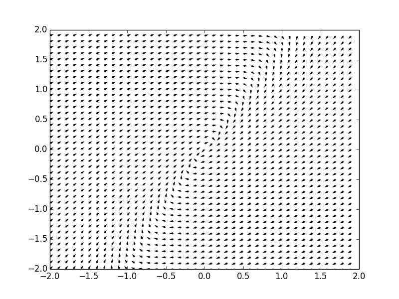
Example. Consider a system of ordinar differential equations
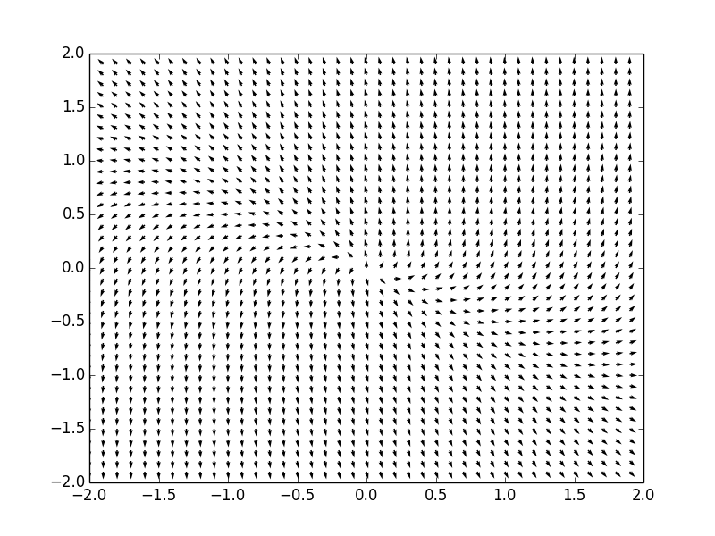
The coefficient matrix \( {\bf A} = \begin{bmatrix} 1&-1 \\ 2&4 \end{bmatrix} \) has two distinct real eigenvalues \( \lambda_1 =3 \) and \( \lambda_2 =2 . \) Therefore, the critical point, which is the origin, is a node point, unstable. We plot the corresponding phase portrait using the following code:
Code:
import numpy as np
import matplotlib.pyplot as plt

def f(Y, t):
    y1, y2 = Y
    return [y1+-1*y2, 2*y1 + 4*y2]
def evaluate():
    r = np.arange(-2, 2, 0.1)
    xgrid = r
    ygrid = r
    X, Y = np.meshgrid(xgrid, ygrid)
    dxdt=X+-1*Y
    dydt=2*X+4*Y
    r = np.sqrt(dxdt**2+dydt**2)
    U=dxdt/r
    V=dydt/r
    plt.quiver(X,Y,U,V)
    plt.xlim((-2,2))
    plt.ylim((-2,2))
    alpha = np.arange(-2,2,0.5)
    plt.show()

evaluate()
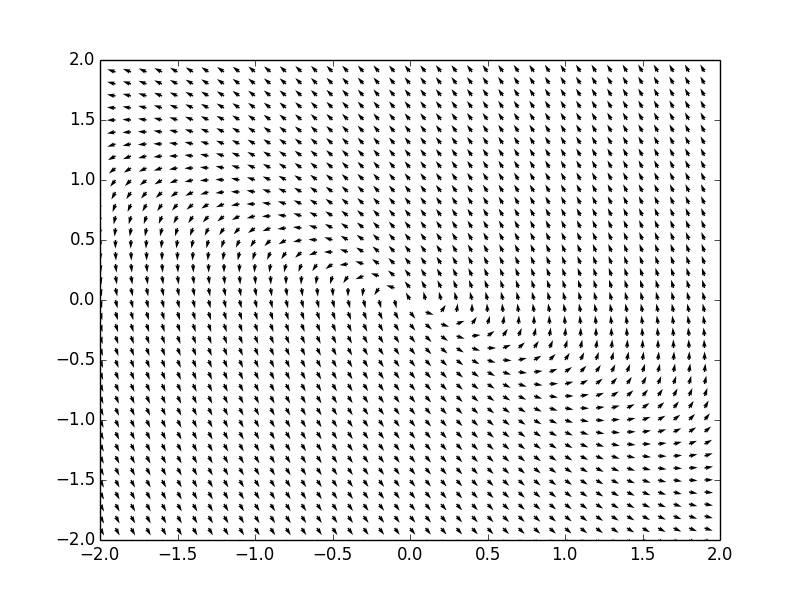
Example. Consider a system of ordinar differential equations
The coefficient matrix \( {\bf A} = \begin{bmatrix} 1&-4 \\ 2&-5 \end{bmatrix} \) has two distinct real eigenvalues \( \lambda_1 =-3 \) and \( \lambda_2 =-1 . \) Therefore, the critical point, which is the origin, is a nodal sink, asymptotically stable. We plot the corresponding phase portrait using the following code:
Code:
import numpy as np
import matplotlib.pyplot as plt

def f(Y, t):
    y1, y2 = Y
    return [y1+-4*y2, 2*y1 + -5*y2]
def evaluate():
    r = np.arange(-2, 2, 0.1)
    xgrid = r
    ygrid = r
    X, Y = np.meshgrid(xgrid, ygrid)
    dxdt=X+-4*Y
    dydt=2*X+-5*Y
    r = np.sqrt(dxdt**2+dydt**2)
    U=dxdt/r
    V=dydt/r
    plt.quiver(X,Y,U,V)
    plt.xlim((-2,2))
    plt.ylim((-2,2))
    alpha = np.arange(-2,2,0.5)
    plt.show()

evaluate()
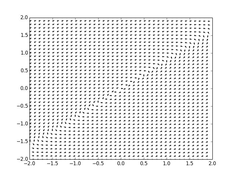
Example. Consider a system of ordinar differential equations
The coefficient matrix \( {\bf A} = \begin{bmatrix} -5&3\\ -3&1 \end{bmatrix} \) has q double real eigenvalue \( \lambda =-2 . \) Therefore, the critical point, which is the origin, is an improper node, asymptotically stable. We plot the corresponding phase portrait using the following code:
Code:
import numpy as np
import matplotlib.pyplot as plt

def f(Y, t):
    y1, y2 = Y
    return [-5*y1+3*y2, -3*y1 + 1*y2]
def evaluate():
    r = np.arange(-2, 2, 0.1)
    xgrid = r
    ygrid = r
    X, Y = np.meshgrid(xgrid, ygrid)
    dxdt=-5*X+3*Y
    dydt=-3*X+Y
    r = np.sqrt(dxdt**2+dydt**2)
    U=dxdt/r
    V=dydt/r
    plt.quiver(X,Y,U,V)
    plt.xlim((-2,2))
    plt.ylim((-2,2))
    alpha = np.arange(-2,2,0.5)
    plt.show()

evaluate()
Example. Consider a system of ordinar differential equations
The coefficient matrix \( {\bf A} = \begin{bmatrix} 1&-4 \\ 1&5 \end{bmatrix} \) has a double real eigenvalue \( \lambda =3 . \) Therefore, the critical point, which is the origin, is an improper node point, unstable. We plot the corresponding phase portrait using the following code:
Code:
import numpy as np
import matplotlib.pyplot as plt

def f(Y, t):
    y1, y2 = Y
    return [1*y1+-4*y2, 4*y1 + 5*y2]
def evaluate():
    r = np.arange(-2, 2, 0.1)
    xgrid = r
    ygrid = r
    X, Y = np.meshgrid(xgrid, ygrid)
    dxdt=-1*X+-4*Y
    dydt=4*X+5*Y
    r = np.sqrt(dxdt**2+dydt**2)
    U=dxdt/r
    V=dydt/r
    plt.quiver(X,Y,U,V)
    plt.xlim((-2,2))
    plt.ylim((-2,2))
    alpha = np.arange(-2,2,0.5)
    plt.show()

evaluate()
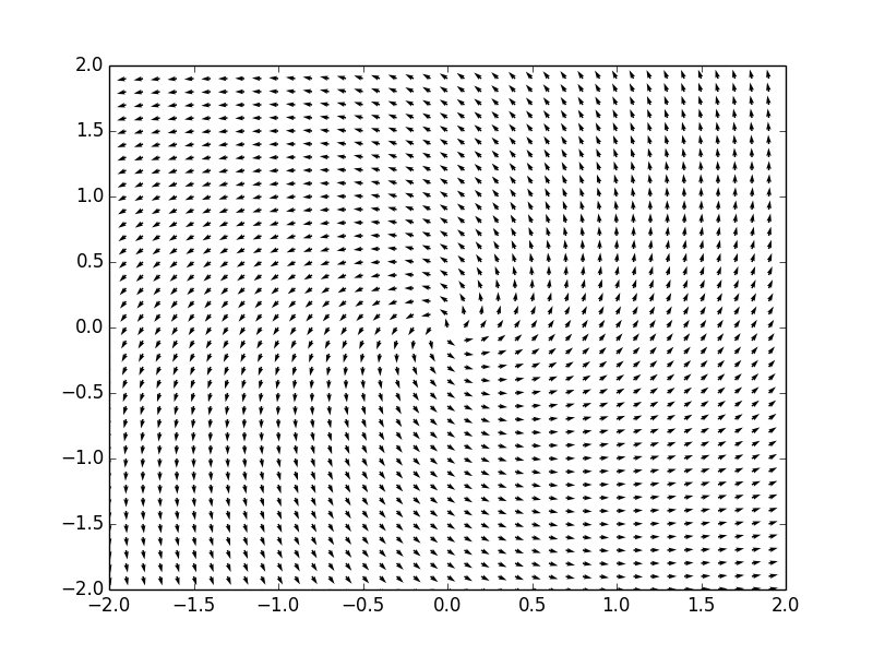
Example. Consider a system of ordinar differential equations
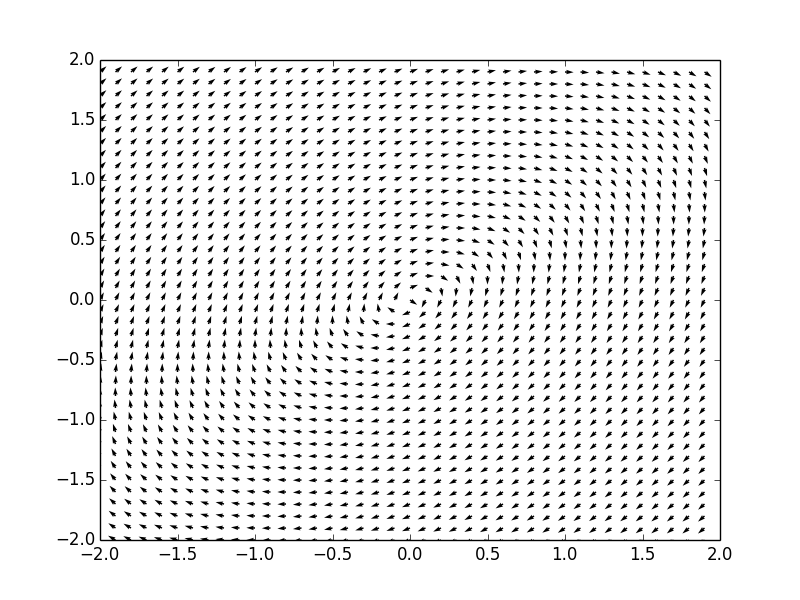
The coefficient matrix \( {\bf A} = \begin{bmatrix} -4&5 \\ -2&2 \end{bmatrix} \) has two complex conjugate eigenvalues \( \lambda_{1,2} = -1 \pm {\bf j} . \) Therefore, the critical point, which is the origin, is a spiral point, asymptotically stable. We plot the corresponding phase portrait using the following code:
Code:
import numpy as np
import matplotlib.pyplot as plt

def f(Y, t):
    y1, y2 = Y
    return [-4*y1+5*y2, -2*y1 + 2*y2]
def evaluate():
    r = np.arange(-2, 2, 0.1)
    xgrid = r
    ygrid = r
    X, Y = np.meshgrid(xgrid, ygrid)
    dxdt=-4*X+5*Y
    dydt=-2*X+2*Y
    r = np.sqrt(dxdt**2+dydt**2)
    U=dxdt/r
    V=dydt/r
    plt.quiver(X,Y,U,V)
    plt.xlim((-2,2))
    plt.ylim((-2,2))
    alpha = np.arange(-2,2,0.5)
    plt.show()

evaluate()
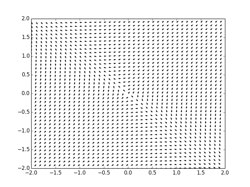
Example. Consider a system of ordinar differential equations
The coefficient matrix \( {\bf A} = \begin{bmatrix} 2&-3 \\ 3&2 \end{bmatrix} \) has two complex conjugate eigenvalues \( \lambda_{1,2} = 2\pm 3{\bf j} . \) Therefore, the critical point, which is the origin, is a spiral point, unstable. We plot the corresponding phase portrait using the following code:
Code:
import numpy as np
import matplotlib.pyplot as plt

def f(Y, t):
    y1, y2 = Y
    return [2*y1+-3*y2, 3*y1 + 2*y2]
def evaluate():
    r = np.arange(-2, 2, 0.1)
    xgrid = r
    ygrid = r
    X, Y = np.meshgrid(xgrid, ygrid)
    dxdt=2*X+-3*Y
    dydt=3*X+2*Y
    r = np.sqrt(dxdt**2+dydt**2)
    U=dxdt/r
    V=dydt/r
    plt.quiver(X,Y,U,V)
    plt.xlim((-2,2))
    plt.ylim((-2,2))
    alpha = np.arange(-2,2,0.5)
    plt.show()

evaluate()
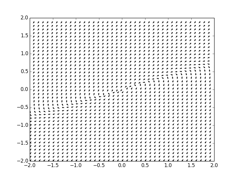
Example. Consider a system of ordinar differential equations
The coefficient matrix \( {\bf A} = \begin{bmatrix} -2&5 \\ -4&2 \end{bmatrix} \) has two distinct real eigenvalues \( \lambda_1 =3 \) and \( \lambda_2 =2 . \) Therefore, the critical point, which is the origin, is a center, stable. We plot the corresponding phase portrait using the following code:
Code:
import numpy as np
import matplotlib.pyplot as plt

def f(Y, t):
    y1, y2 = Y
    return [-2*y1+5*y2, -4*y1 + 2*y2]
def evaluate():
    r = np.arange(-2, 2, 0.1)
    xgrid = r
    ygrid = r
    X, Y = np.meshgrid(xgrid, ygrid)
    dxdt=-2*X+5*Y
    dydt=-4*X+2*Y
    r = np.sqrt(dxdt**2+dydt**2)
    U=dxdt/r
    V=dydt/r
    plt.quiver(X,Y,U,V)
    plt.xlim((-2,2))
    plt.ylim((-2,2))
    alpha = np.arange(-2,2,0.5)
    plt.show()

evaluate()